Which Inter-Rater Reliability Coefficient Should You Use?

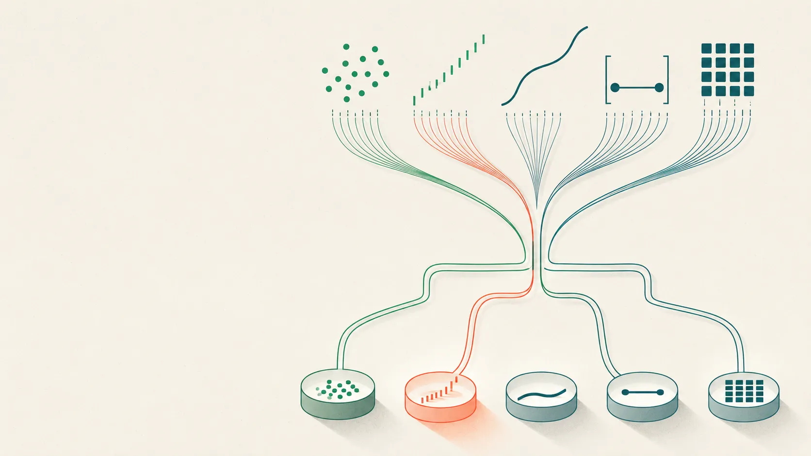
Which inter-rater reliability coefficient you should use is decided almost entirely by three facts about your data: what kind of labels you collected, how many people did the labeling, and whether anyone skipped items. Get those three right and the choice is close to mechanical; get them wrong and you can report a number that flatters bad data or punishes good data. The stakes are concrete: under a skewed label, two coders can agree 84% of the time and still post a Cohen’s kappa near 0.11, while Gwet’s AC1 on the same table reads 0.80 (Gwet, 2008). This guide is a decision tree, not a lecture—one table that maps data type, rater count, and missingness to the coefficient that fits, then the reasoning and failure mode behind each cell.

What determines which agreement coefficient you need?

Three properties of your data decide the coefficient, in this order: the measurement level of the labels, the number of raters, and whether the design has missing ratings. A fourth property, how lopsided the category frequencies are, decides whether the chance correction behaves. Hallgren (2012) organizes the whole choice around exactly these axes, and treating them as a checklist removes most of the guesswork.

The order matters because each axis narrows the field. Data type rules out whole families at once—an intraclass correlation is wrong for nominal labels, and a nominal kappa throws away the ordering in a severity scale. Rater count then splits the survivors into the two-rater and many-rater cases. Missing data and prevalence are the tie-breakers that push you toward the coefficients built to absorb them.

The inter-rater reliability decision table

The table below is the whole guide compressed: find the row that matches your data type, rater count, and missingness, and read off the coefficient. Everything after it is the reasoning behind a cell. This is a starting recommendation, not a verdict—report the coefficient with a confidence interval and the base rates so a reader can judge it (Gwet, 2008).

Your data	Raters	Missing data?	Recommended coefficient	Why
Nominal (unordered categories)	Exactly 2	No	Cohen's kappa	Chance-corrected agreement; the default reviewers expect (Cohen, 1960)
Nominal	3 or more	No	Fleiss' kappa (or Krippendorff's alpha)	Generalizes kappa to many raters (Fleiss, 1971)
Nominal, one category dominant	2 or more	Any	Gwet's AC1	Paradox-resistant where kappa collapses (Gwet, 2008)
Ordinal (severity ratings)	Exactly 2	No	Weighted kappa (linear or quadratic)	Penalizes far disagreements more than near ones
Ordinal	3 or more, or gaps	Yes	Ordinal Krippendorff's alpha	Many raters, missing cells, distance-weighted (Krippendorff, 2004)
Interval / continuous scores	2 or more	Handled	Intraclass correlation (ICC)	Correlation for continuous ratings (Shrout & Fleiss, 1979)
Any level, many raters, gaps	3 or more	Yes	Krippendorff's alpha	The general case; one formula covers it (Krippendorff, 2004)
Spatial masks (pixels)	Any	—	Dice / IoU (not a kappa)	Region overlap, not category agreement
Text spans (NER, segments)	Any	—	Span-level F1 / IoU	Boundary plus label, not a single coefficient

The three families that trip people up sit in the last rows. Spatial and span data are not a chance-corrected-coefficient problem at all, which the sections below make concrete.

Why is data type the first fork?

Data type comes first because the measurement level of your labels determines what a disagreement even means, and every coefficient encodes an assumption about that. A nominal coefficient treats “mild” versus “severe” as the same size of miss as “mild” versus “moderate”—it only asks whether the labels match. That is correct for unordered categories like speaker role, and badly wrong for a graded severity rating.

The five families you will meet in practice map cleanly onto tools. Nominal and ordinal categories are kappa-and-alpha territory. Interval or continuous scores belong to the intraclass correlation. Spatial masks and text spans leave the world of category agreement entirely, because the disagreement is about where a boundary sits, not which label a fixed item gets.

Ordinal data is the family most often mishandled. Rating an item “mild” when a colleague rated it “moderate” is a small disagreement; “none” versus “severe” is a large one. A plain nominal kappa charges both the same, which understates real agreement on a scale. Weighted kappa and ordinal alpha fix this by weighting each disagreement by how far apart the two ratings are (Krippendorff, 2004).

Cohen vs Fleiss vs Krippendorff: how many raters?

Rater count splits the nominal and ordinal families in two. Cohen’s kappa is defined for exactly two raters (Cohen, 1960). The moment a third rater joins, or ratings go missing, you need a coefficient built for the general case, and this is where the cohen vs fleiss vs krippendorff question is usually settled.

Fleiss’ kappa generalizes kappa to any fixed number of raters on nominal categories, which is why it shows up in reliability studies with a panel of coders (Fleiss, 1971). Its constraints are the tell: it still assumes nominal labels and complete data. Krippendorff’s alpha lifts all three limits at once—any number of raters, any measurement level, and missing data—by computing chance from the pooled distribution of every value rather than from each rater’s individual habits (Krippendorff, 2004).

Property	Cohen's kappa	Fleiss' kappa	Krippendorff's alpha
Number of raters	Exactly 2	Any fixed number	Any number
Measurement level	Nominal	Nominal	Nominal, ordinal, interval, ratio
Missing data	Not allowed	Not allowed	Handled natively
Chance model	Each rater's marginals	Pooled category rates	Pooled distribution of all values
Reach for it when	Two coders, clean data	A panel, clean nominal data	Anything more realistic

For the full mechanics of the two-rater case, see our guide to computing and interpreting Cohen’s kappa; for the many-rater, missing-data case worked by hand and in code, see Krippendorff’s alpha, computed.

Is percent agreement ever enough?

Percent agreement is a useful companion and a dangerous headline. It is easy to read—the share of items two raters labeled the same way—but it credits agreement that would happen by chance, so it flatters skewed data. Two raters who both mark a common feature present nine times in ten will agree most of the time without looking, and raw percent agreement rewards them for it.

Report percent agreement alongside a chance-corrected coefficient, never in its place. The gap between the two is informative: a large gap means chance is doing much of the work, which is your early warning that prevalence is skewed and that the coefficient you pick next matters more than usual. The worked example below shows exactly that gap.

The kappa paradox: when to switch to Gwet’s AC1

Cohen’s and Fleiss’ kappa share a failure mode called the kappa paradox: when one category dominates, agreement can be high while kappa is low or even near zero (Feinstein & Cicchetti, 1990). The cause is the chance correction. Kappa estimates expected agreement from the raters’ marginals, and under extreme prevalence that estimate approaches the observed agreement, so the numerator shrinks toward zero and kappa follows.

Gwet’s AC1 was built to survive this. It keeps the chance-corrected form but replaces kappa’s chance-agreement term with one that does not inflate as a category gets rare, which keeps the coefficient stable under the same skew that breaks kappa (Gwet, 2008). The practical rule: when a label’s base rate is far from 50%, compute AC1 next to kappa and report both. If they diverge sharply, the paradox is present and AC1 is the more honest summary.

Ordinal data: weighted kappa or ordinal alpha?

For ordered categories, use a coefficient that counts distance, not just match or mismatch. Weighted kappa is the two-rater tool: linear weights penalize a disagreement in proportion to how many steps apart the ratings are, and quadratic weights penalize larger gaps far more heavily. A one-step slip on a severity scale should not cost the same as a three-step one, and weighting is how that intuition enters the number.

Ordinal Krippendorff’s alpha does the same job for more than two raters and for missing data, by swapping in an ordinal distance function while the rest of the formula stays fixed (Krippendorff, 2004). Clinician-rated severity scales are the canonical case. The Montgomery-Åsberg Depression Rating Scale (MADRS) and Andreasen’s Scale for the Assessment of Thought, Language and Communication (TLC) both produce ordinal per-item ratings, where a distance-weighted coefficient is the honest measure of how well two raters agree.

Continuous ratings: which intraclass correlation?

For continuous or interval-scaled ratings—a total scale score, a reaction time, a count—use an intraclass correlation coefficient, not kappa. The ICC measures how much of the total variance is due to real differences between subjects rather than to disagreement between raters (Shrout & Fleiss, 1979). The catch is that “the ICC” is a family, and the forms give different numbers on the same data.

Choosing among them comes down to two decisions: the model (are the same raters used for every subject, and are they a fixed set or a random sample?) and the definition (do you care about absolute agreement, or only consistency of ranking?). Koo and Li (2016) give a selection guideline and a benchmark worth quoting in full:

“Values less than 0.5 are indicative of poor reliability, values between 0.5 and 0.75 indicate moderate reliability, values between 0.75 and 0.9 indicate good reliability, and values greater than 0.90 indicate excellent reliability.”

The one rule that prevents most confusion: state which ICC form you computed, because a reader cannot interpret the value without it (Koo & Li, 2016).

Spans and pixels: when agreement isn’t a coefficient at all

Some annotation tasks are not category-agreement problems, and forcing a kappa onto them gives a misleading number. When two coders segment a pixel mask, the question is how much their regions overlap, which is a Dice or Intersection-over-Union score, not a chance-corrected coefficient. A per-pixel kappa collapses here for the same reason as the paradox: the background class dominates, so chance agreement is nearly total. The mechanics are in our guide to image-segmentation agreement with Dice, IoU, and STAPLE.

Text spans sit between the two worlds. Marking where a phenomenon occurs in a transcript is a boundary problem, scored with span-level F1 or token IoU, because two coders can flag the same passage yet disagree on its exact start and end. Deciding what label the span gets is back to categorical agreement, kappa’s home turf. A span-annotation project usually needs both a boundary metric and a category coefficient, reported separately, so a boundary disagreement never masquerades as a labeling one.

A worked example: same data, three very different numbers

Here is the paradox in one synthetic table. Two coders each judge 100 utterances for a common feature—present or absent—that turns out to be present about 90% of the time.

	Coder B: present	Coder B: absent	Row total
Coder A: present	82	8	90
Coder A: absent	8	2	10
Column total	90	10	100

Percent agreement is the diagonal: (82 + 2) / 100 = 0.84. Cohen’s kappa corrects for chance using the marginals: expected agreement is Pₑ = 0.90·0.90 + 0.10·0.10 = 0.82, so κ = (0.84 − 0.82) / (1 − 0.82) = 0.11. Gwet’s AC1 uses a chance term that does not inflate with prevalence: Pₑ = 2·0.90·0.10 = 0.18, so AC1 = (0.84 − 0.18) / (1 − 0.18) = 0.80. By the widely used Landis and Koch (1977) bands, κ = 0.11 counts as only “slight” agreement while AC1 = 0.80 is “almost perfect”—the same table, two opposite verdicts.

The three numbers describe one dataset. Percent agreement overstates, kappa understates because of the skew, and AC1 lands where a human would: these coders mostly agree, but on a lopsided label that agreement is hard to prove with kappa. Report all three under skewed prevalence and the disagreement between them tells the real story.

Common mistakes when choosing a coefficient

Most reporting errors come from picking the coefficient by habit rather than by data type. A handful account for the majority.

• Using nominal kappa on an ordinal scale. It discards the ordering and understates agreement; use weighted kappa or ordinal alpha instead.
• Trusting a low kappa under skewed prevalence. Check the base rates and compute Gwet’s AC1 before concluding your coders disagree (Feinstein & Cicchetti, 1990).
• Reporting an ICC without its form. The value is uninterpretable unless you state the model and definition (Koo & Li, 2016).
• Forcing a coefficient onto spans or pixels. Overlap tasks need F1, IoU, or Dice, not a chance-corrected category statistic.
• Reporting a bare number. Give the coefficient with a confidence interval, the rater count, and the category frequencies, so the estimate can be judged (Gwet, 2008).

Which inter-rater reliability coefficient should you use?

Start from the data, not the coefficient you already know. Which inter-rater reliability coefficient fits is a short walk down the table: name the data type, count the raters, check for missing cells, and glance at the base rates. Two raters and unordered categories give Cohen’s kappa; a panel gives Fleiss’ kappa or Krippendorff’s alpha; ordinal ratings add distance weighting; continuous scores hand off to an ICC; a dominant category calls for Gwet’s AC1; and spans or pixels leave coefficients behind for F1, IoU, or Dice.

In Tagaroo, each coding scheme runs as a live annotation workflow, and inter-rater reliability is computed as coders work, with the coefficient matched to the scale’s measurement level—ordinal scales get a distance-weighted statistic, nominal span labels get the nominal form. Pick the instrument for the question, not the other way round: that is the difference between a number and a defensible reliability claim.

References

• Cohen, J. (1960). A coefficient of agreement for nominal scales. Educational and Psychological Measurement, 20(1), 37–46. doi.org/10.1177/001316446002000104
• Fleiss, J. L. (1971). Measuring nominal scale agreement among many raters. Psychological Bulletin, 76(5), 378–382. doi.org/10.1037/h0031619
• Landis, J. R., & Koch, G. G. (1977). The measurement of observer agreement for categorical data. Biometrics, 33(1), 159–174. doi.org/10.2307/2529310
• Shrout, P. E., & Fleiss, J. L. (1979). Intraclass correlations: uses in assessing rater reliability. Psychological Bulletin, 86(2), 420–428. doi.org/10.1037/0033-2909.86.2.420
• Feinstein, A. R., & Cicchetti, D. V. (1990). High agreement but low kappa: I. The problems of two paradoxes. Journal of Clinical Epidemiology, 43(6), 543–549. doi.org/10.1016/0895-4356(90)90158-L
• Krippendorff, K. (2004). Reliability in content analysis: some common misconceptions and recommendations. Human Communication Research, 30(3), 411–433. doi.org/10.1111/j.1468-2958.2004.tb00738.x
• Gwet, K. L. (2008). Computing inter-rater reliability and its variance in the presence of high agreement. British Journal of Mathematical and Statistical Psychology, 61(1), 29–48. doi.org/10.1348/000711006X126600
• Hallgren, K. A. (2012). Computing inter-rater reliability for observational data: an overview and tutorial. Tutorials in Quantitative Methods for Psychology, 8(1), 23–34. doi.org/10.20982/tqmp.08.1.p023
• Koo, T. K., & Li, M. Y. (2016). A guideline of selecting and reporting intraclass correlation coefficients for reliability research. Journal of Chiropractic Medicine, 15(2), 155–163. doi.org/10.1016/j.jcm.2016.02.012