Dice vs IoU vs Hausdorff: Segmentation Metrics Explained
Dice vs IoU, the Jaccard index, and Hausdorff distance compared: formulas, the Dice-IoU identity, and when overlap metrics mislead. See which to report.
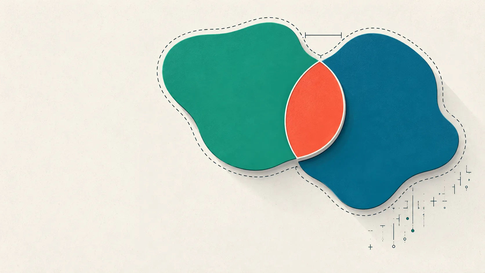
Dice vs IoU is the first fork every segmentation project reaches, and the honest answer is that the two barely differ: both measure how much your predicted mask overlaps the ground truth, and both rank your models in exactly the same order. The Dice coefficient and the Jaccard index (IoU) are two views of one quantity, related by a fixed identity. Where segmentation evaluation actually goes wrong is elsewhere: overlap metrics quietly mislead on small structures and hide boundary errors on large ones, which is why the Hausdorff distance exists. This guide gives the exact formulas, the conversion between them, and a clear rule for when each metric earns its place.
Dice vs IoU: what’s the difference?
Dice vs IoU comes down to how each formula scales the same overlap: Dice counts the shared region twice, IoU counts the union once. Both take two sets, the predicted mask A and the ground-truth mask B, and reward their intersection. Neither cares about the shape of the error, only its area.
Both range from 0 (no overlap) to 1 (identical masks). The one durable difference: for any partial overlap, Dice is larger than IoU, because doubling the intersection in the numerator outweighs the denominators. They meet only at the endpoints, 0 and 1. So a reported Dice of 0.90 and an IoU of 0.90 are not comparable scores, and quoting one without saying which you used is a common source of confusion across papers.
How do you convert between Dice and IoU?
You convert with a fixed algebraic identity, no data required: Dice = 2·IoU / (1+IoU), and inverting it, IoU = Dice / (2−Dice). The relationship is monotonic, which is the practically important part: whichever model has the higher IoU also has the higher Dice, so the two never disagree about which segmentation is better.
Work one synthetic case. Suppose the intersection of the two masks is 90 pixels, and each mask covers 100 pixels, so the union is 100 + 100 − 90 = 110. Dice = 2·90 / (100+100) = 0.90, and IoU = 90 / 110 = 0.818.
Check the identity: 2·0.818 / (1+0.818) = 0.90. The gap between 0.90 and 0.818 is the whole story of Dice vs IoU, one overlap under two scalings.
| Metric | Formula | Range | What it captures | Main weakness |
|---|---|---|---|---|
| Dice (DSC) | 2·|A∩B| / (|A|+|B|) | 0 to 1 (1 = perfect) | Region overlap; equals the F1 score | Size-sensitive; blind to boundary shape |
| IoU (Jaccard) | |A∩B| / |A∪B| | 0 to 1 (1 = perfect) | Region overlap; penalizes error slightly harder | Same blind spots as Dice |
| Hausdorff (HD) | max nearest-surface distance | 0 to ∞ (0 = perfect) | Worst-case boundary error | Dominated by a single outlier voxel |
| HD95 / ASSD | 95th-percentile / mean surface distance | 0 to ∞ (0 = perfect) | Typical boundary error | Needs voxel spacing; ignores region overlap |
What is the Dice coefficient?
The Dice similarity coefficient (DSC), also called the Sørensen–Dice coefficient, is the ratio of twice the overlap to the total size of both masks: 2·|A∩B| / (|A|+|B|). In classification terms it is identical to the F1 score, the harmonic mean of precision and recall, because both collapse to 2·TP / (2·TP + FP + FN) (Taha & Hanbury, 2015). That is why the same number shows up under two names depending on whether the author came from imaging or from machine learning.
Dice is the default reported metric in most medical-segmentation work, and for good reason: it is intuitive, bounded, and forgiving enough to produce readable numbers on hard tasks. Its forgiveness is also its trap, which the limitations section below makes concrete.
What is IoU, the Jaccard index?
The Intersection over Union (IoU), known in statistics as the Jaccard index, is the overlap divided by the union of the two masks: |A∩B| / |A∪B| (Taha & Hanbury, 2015). It is the standard overlap metric in computer-vision detection and segmentation benchmarks, where a prediction is often counted as a hit only if its IoU with the ground truth clears a threshold such as 0.5.
Because the union sits in the denominator, IoU penalizes a given error slightly harder than Dice does, so its numbers run lower. For Jaccard index segmentation reporting the choice between IoU and Dice is cosmetic as long as you are consistent, since the two rank identically. Pick one, name it explicitly, and use it throughout.
When do overlap metrics mislead?
Overlap metrics mislead in two situations: small or thin structures, and boundary errors on large objects. Both follow from the same fact, that Dice and IoU measure area, so their sensitivity depends on how big the target is.
The size problem is easiest to see with numbers. Take a 10-pixel structure where your model gets 8 pixels right, misses 2, and adds 2 false ones: Dice = 2·8 / (10+10) = 0.80. Now make the exact same four-pixel error on a 1,000-pixel structure: Dice = 2·998 / (1000+1000) = 0.998. Identical mistakes, wildly different scores.
The mirror-image failure is a boundary error hiding inside a high score. Add a one-voxel-thick rind around a large organ and Dice can still read above 0.98, even though the contour, the thing a surgeon or a downstream measurement depends on, is systematically off. As the Metrics Reloaded consortium put it, “chosen performance metrics often do not reflect the domain interest,” and they warn that “flaws in machine learning (ML) algorithm validation are an underestimated global problem” (Maier-Hein et al., 2024). The guideline literature reaches the same conclusion by a different route: Dice, Jaccard, sensitivity, specificity, Cohen’s kappa, and Hausdorff distance each capture a different facet, and reporting one in isolation is a known source of statistical bias (Müller, Soto-Rey & Kramer, 2022).
What is Hausdorff distance, and what are HD95 and ASSD?
The Hausdorff distance is a boundary metric: it is the largest distance from any point on one mask’s surface to the nearest point on the other’s, taken symmetrically. Where Dice and IoU ask “how much overlaps?”, Hausdorff asks “how far is the worst-placed boundary point?” It is measured in millimeters (given voxel spacing), and lower is better, with 0 meaning the contours match exactly.
Its strength, sensitivity to the single worst point, is also its weakness: one stray voxel far from the object can blow up the whole number. Taha and Hanbury (2015) flag this outlier sensitivity directly and recommend more stable variants. The two you will see most often are HD95, the 95th percentile of surface distances rather than the strict maximum, which discards the top few outliers, and the average symmetric surface distance (ASSD), the mean boundary error in both directions. HD95 has become the de facto boundary metric in medical-imaging challenges precisely because it keeps Hausdorff’s contour awareness without letting one noisy voxel dominate.
The practical rule that follows: report a region metric and a boundary metric together. Dice or IoU tells you whether you found the object; HD95 or ASSD tells you whether you traced its edge. Metrics Reloaded frames metric choice around a “problem fingerprint,” selecting from the task rather than from habit, and pairing overlap with boundary distance is the most common instance of that advice (Maier-Hein et al., 2024).
Where does Cohen’s kappa fit, and why does it collapse on pixels?
Cohen’s kappa is the right tool for categorical agreement, but the wrong tool for pixels. Kappa measures how often two raters assign the same category beyond what chance would produce, using the Landis and Koch (1977) bands where values above 0.81 read as almost perfect. That chance correction is exactly what breaks it on segmentation.
Treat a segmentation as a per-pixel “object vs background” classification and the background class swamps everything, often 95% or more of the image. When one class dominates, two raters agree most of the time by accident, so kappa subtracts nearly all of that agreement away and can read near zero even for a visibly good mask, the same class-imbalance trap known as the kappa paradox. That instability is why the segmentation literature reaches for Dice and IoU instead of a chance-corrected category statistic (Müller, Soto-Rey & Kramer, 2022). If your labels really are categories rather than regions, kappa is appropriate, and our guide to computing and interpreting Cohen’s kappa covers when to use weighted kappa or Krippendorff’s alpha instead.
How does this map to transcript annotation?
The overlap-versus-category split is not unique to images; it reappears the moment two people annotate the same text. Marking where something occurs in a transcript is a span-overlap problem, the one-dimensional cousin of IoU: two coders who both flag a passage but disagree on its exact start and end have partial overlap, scored the same way as two masks. Deciding what label a passage gets is a categorical-agreement problem, which is kappa’s home turf.
Both show up in clinical coding. Tagging the exact stretch of disorganized speech against the TLC scale is a boundary-and-overlap question, where character or token overlap plays the role Dice and IoU play for pixels. Rating overall depression severity against the MADRS is a categorical judgment, where chance-corrected agreement is the honest measure.
For the broader picture of how image and text annotation relate, see the medical image annotation guide and the overview of image annotation types. Tagaroo works on the language side of that split: it turns a coding scheme into guided span annotation with inter-rater reliability computed as coders work, a different job from labeling pixels.
Which segmentation metric should you use?
Pick the metric from the question you are actually asking. Most projects should report at least two.
- Report Dice (or IoU) as your overlap score. They rank models identically, so use whichever your field expects and name it explicitly. IoU is standard in computer-vision benchmarks; Dice dominates medical imaging.
- Add HD95 or ASSD whenever boundaries matter. Thin structures, tubular anatomy, and any task where the contour drives a downstream measurement need a boundary metric, because a high Dice can hide a wrong edge.
- Watch structure size. If your targets vary in size or many are small, expect overlap scores to swing hard, and consider reporting per-size or normalized results (Maier-Hein et al., 2024).
- Don’t reach for Cohen’s kappa on pixels. The background class makes it unstable; save kappa for genuinely categorical labels.
The practical upshot of Dice vs IoU: the two are interchangeable up to a known transformation, so the real decision is not which overlap metric to pick but whether overlap alone is enough. It rarely is. Pair a region metric with a boundary metric, keep an eye on structure size, and you will catch the failures a single Dice score is built to hide.
References
- Maier-Hein, L., Reinke, A., Godau, P., et al. (2024). Metrics reloaded: recommendations for image analysis validation. Nature Methods, 21, 195–212. doi.org/10.1038/s41592-023-02151-z
- Müller, D., Soto-Rey, I., & Kramer, F. (2022). Towards a guideline for evaluation metrics in medical image segmentation. BMC Research Notes, 15, 210. doi.org/10.1186/s13104-022-06096-y
- Taha, A. A., & Hanbury, A. (2015). Metrics for evaluating 3D medical image segmentation: analysis, selection, and tool. BMC Medical Imaging, 15, 29. doi.org/10.1186/s12880-015-0068-x
- Landis, J. R., & Koch, G. G. (1977). The measurement of observer agreement for categorical data. Biometrics, 33(1), 159–174. doi.org/10.2307/2529310
Frequently asked questions
- Is the Dice coefficient the same as the F1 score?
- Yes. For binary segmentation the Dice similarity coefficient equals the F1 score, the harmonic mean of precision and recall, because both reduce to 2·TP / (2·TP + FP + FN) (Taha & Hanbury, 2015). That equivalence is why teams coming from classification and teams coming from imaging often report the same number under two names.
- Why is Dice always higher than IoU?
- Because Dice = 2·IoU / (1+IoU), which is larger than IoU for every value strictly between 0 and 1; the two coincide only at 0 and at 1. They also rank results identically, so a model that wins on Dice wins on IoU (Taha & Hanbury, 2015). The gap is widest in the mid-range, around IoU 0.5, where Dice reads about 0.67.
- When should I report Hausdorff distance instead of Dice?
- Report a boundary metric such as the Hausdorff distance, or its 95th-percentile variant HD95, when contour accuracy matters more than bulk overlap, for example thin or tubular structures and surgical margins, because overlap metrics can stay high while the boundary is visibly wrong (Maier-Hein et al., 2024; Taha & Hanbury, 2015).
- Which metrics should a medical-imaging segmentation paper report?
- Current guidance is to choose metrics from the task rather than habit, and to pair a region-overlap metric (Dice or IoU) with a boundary metric (HD95 or average surface distance) instead of reporting Dice alone (Maier-Hein et al., 2024; Müller, Soto-Rey & Kramer, 2022).
- Can I use Cohen's kappa to score a segmentation?
- It is a poor fit. On a pixel map the background class dominates, so chance agreement is nearly total and kappa becomes unstable, often collapsing toward zero even for a good mask (Landis & Koch, 1977; Müller, Soto-Rey & Kramer, 2022). That skew is why segmentation uses overlap metrics like Dice and IoU rather than a chance-corrected category statistic.
Keep reading
 Image & Multimodal Annotation
Medical Image Annotation: A Complete Guide for AI Teams
Medical image annotation, end to end: annotation types, who should label, consensus and adjudication, DICOM de-identification, and QA tied to risk.
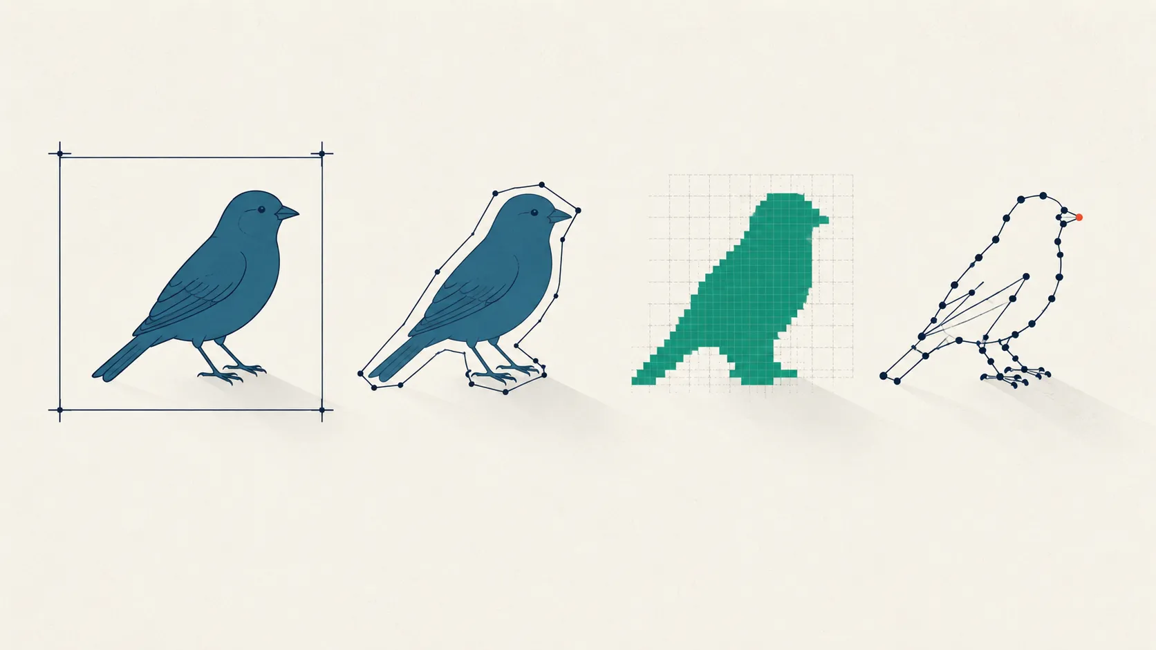 Image & Multimodal Annotation
Image Annotation Types: Cost vs Precision, Explained
Bounding box, polygon, semantic vs instance vs panoptic masks, or keypoints? Compare image annotation types by cost, precision, and downstream task.
 Reliability & Agreement
Cohen's Kappa: How to Compute and Interpret Agreement
How to compute Cohen's kappa and weighted kappa by hand, read the result honestly, and know when to use Krippendorff's alpha, ICC, or Gwet's AC1 instead.
Put this into practice
Tagaroo turns any rating scale or coding scheme into a guided annotation workflow—with inter-rater reliability computed as you go.