Geospatial Image Annotation: Labeling Beyond the Everyday
Geospatial image annotation covers satellite, aerial, and microscopy imagery—where huge rasters, rare classes, and expert-only labels change the rules.
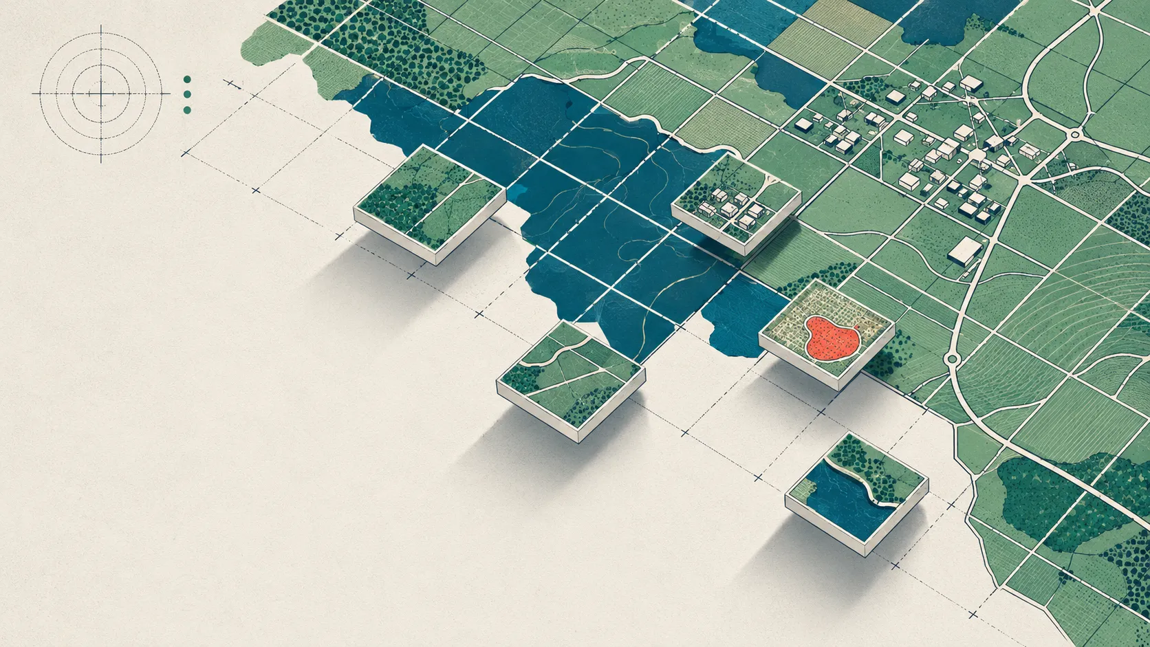
Geospatial image annotation is the same discipline as labeling everyday photos—draw a boundary, attach a class, check that two people agree—stretched until the familiar rules snap. The images are too large to open at once, the objects that matter are the rarest ones in the frame, every pixel carries a real-world coordinate, and the person who can label correctly often holds a doctorate in the subject.
That gap is why a workflow tuned for cats-and-dogs bounding boxes struggles on a satellite scene or a microscopy stack. This piece walks the differences that actually bite—multi-scale rasters, georeferencing, class imbalance, and expert-only labels—across satellite and aerial imagery, microscopy and cell counting, and natural-world science, with the datasets and numbers behind each.
What is geospatial image annotation?
Geospatial image annotation is the labeling of satellite, aerial, or drone imagery so that features on the ground—buildings, roads, land-cover types, flooded areas—become structured data tied to real-world coordinates. Scientific image annotation extends the same idea to microscopy, astronomy, and other instrument imagery, where the labels feed measurement and discovery rather than a consumer product.
The unit of work is familiar: a region of an image plus a class from a defined scheme. What changes is everything around that unit. The image is a georeferenced raster, not a snapshot; the scheme is a land-cover legend or a cell-type list written by specialists; and the annotator is reading a signal, not recognizing an object. This is why the field goes by so many names—satellite image labeling, remote sensing annotation, microscopy image annotation—that all describe the same expert-driven discipline.
How does geospatial image annotation differ from everyday photo labeling?
Geospatial image annotation differs on four axes at once: the images are enormous and multi-scale, every pixel is georeferenced, the classes are long-tailed, and the labelers must be domain experts. Any single one of these is manageable. Together they change tooling, sampling, cost, and quality control, which is why lifting a consumer-photo pipeline onto scientific data rarely works unchanged.
| Challenge | Everyday photo labeling | Geospatial & scientific imagery | What it changes |
|---|---|---|---|
| Image size and scale | A few megapixels, a single scale | Rasters 10,000+ pixels a side; objects from one pixel to whole-scene | Tiling, multi-resolution schemes (BigEarthNet varies patch size by band; Sümbül et al., 2019) |
| Coordinates | Pixel coordinates only | Every pixel has a real-world position (georeferencing) | Labels are geospatial features with projection and coordinates, not just boxes |
| Class balance | Roughly even classes | Long-tailed; the rare event carries the value | Uniform sampling starves rare classes (iNaturalist is imbalanced on purpose; Van Horn et al., 2018) |
| Who can label | Most literate adults | Domain experts: analysts, radiologists, cell biologists | Small labeler pools, higher cost, consensus among few (CTC gold truth uses three experts; Maška et al., 2023) |
Whether the right label is a bounding box, a polygon, or a per-pixel mask still depends on the question you are asking, the same menu of image annotation types that governs any vision dataset. The difference is that here the menu is applied at a scale, and by a labeler, that everyday projects never see.
How do you label satellite and aerial imagery?
You label satellite and aerial imagery by tiling a large georeferenced raster into manageable chips, then marking ground features as polygons (building footprints, parcels), lines (roads, rivers), or per-pixel land-cover masks. Because the label is a geospatial feature, it inherits coordinates, projection, and scale from the source image, so a “building” is not a box on a screen but a footprint on the Earth.
SpaceNet is the canonical corpus for this work. Its partners released a large body of labeled satellite imagery on AWS, running public challenges first on building-footprint extraction and later on road networks, motivated by a blunt observation: updating foundational maps “is currently a highly manual process requiring a large number of human labelers” (Van Etten et al., 2018). That sentence is the whole economic case for better remote sensing annotation.
Scale and diversity are the other tax. xView bounding-boxed over 1 million objects across 60 classes in more than 1,400 km² of 0.3 m WorldView-3 imagery, using a bespoke process with three stages of quality control (Lam et al., 2018). The classes range from small vehicles to large buildings in the same frame, which is the multi-scale problem in one dataset.
Land cover adds another wrinkle: a single chip can belong to several classes at once. BigEarthNet annotates 590,326 Sentinel-2 patches with multiple land-cover labels drawn from the CORINE Land Cover 2018 database, and crucially the patch dimensions differ by band—120 pixels a side for 10 m bands, 60 for 20 m, 20 for 60 m (Sümbül et al., 2019). Multi-scale is not a nuisance here; it is baked into the sensor.
For the annotation protocol itself, urban-scene work transfers cleanly to aerial imagery segmentation. Cityscapes built its 5,000 fine masks as layered polygons drawn back-to-front so no boundary is marked twice, then ran a two-tier strategy: over 1.5 hours per image for fine labels and under 7 minutes for coarse ones, trading boundary accuracy for volume (Cordts et al., 2016). The same layered-polygon, tiered-effort discipline is exactly what a large land-cover project needs.
Because these masks are compared pixel-for-pixel, the agreement metrics are the segmentation ones—Dice, IoU, and Hausdorff distance—not a flat accuracy that the dominant background class would inflate.
What makes microscopy and cell annotation so labor-intensive?
Microscopy image annotation is slow because a single field can hold hundreds of overlapping cells with fuzzy boundaries, and only a trained biologist can call them correctly. So the gold standard is built from a handful of experts, not a crowd, and it never covers everything.
The Cell Tracking Challenge makes the cost visible. Its gold-truth segmentation is the majority opinion among three independent expert annotators per video, and that triplet is also how the challenge measures inter-annotator variability (Maška et al., 2023). Even so, that gold-truth segmentation reaches only about 17.8% of cells on average, “due to the labor-intensive nature of manual annotations.”
To close that gap, the challenge fuses the outputs of top-performing algorithms into a ‘silver truth’ that reaches roughly 99% coverage (Maška et al., 2023). That fusion is model-assisted labeling and consensus estimation working together, the same idea as STAPLE, which estimates a probabilistic consensus and each annotator’s reliability rather than counting votes equally (Warfield et al., 2004). The identical expert-consensus problem shows up in clinical imaging, which we treat in the medical image annotation guide.
Why do rare classes and class imbalance break standard labeling?
Rare classes break standard labeling because the events you most need to find—a new lesion type, an uncommon mineral, an endangered species, a collapsed building—are a tiny fraction of the data, and uniform sampling barely surfaces them. iNaturalist was built to expose exactly this failure.
The dataset is deliberately long-tailed: 859,000 images across more than 5,000 species, mirroring a natural world where “some species are more abundant and easier to photograph than others” (Van Horn et al., 2018). The authors report the predictable consequence—models show “poor results for classes with small numbers of training examples,” so the tail is where accuracy goes to die.
For annotation, that reshapes the plan. You cannot sample uniformly and expect the rare class to appear, so you oversample the regions or time windows where it occurs and mine hard cases with a model in the loop. And a class with five examples cannot support a stable reliability estimate, which forces you to report agreement per class rather than in aggregate. Getting that class scheme right up front is its own skill, covered in designing a label taxonomy.
Who is qualified to label scientific images?
Often only a domain expert. Reading a satellite scene, a histology slide, or a fluorescence stack is a trained skill, so the labeler pool is small, expensive, and itself a source of disagreement that has to be measured rather than assumed away.
This is the opposite of the crowd-scale economics that make everyday labeling cheap. General annotators handle everyday classes well, but scientific labels need specialists, which is why benchmarks like the Cell Tracking Challenge lean on two or three experts and then quantify how much they diverge (Maška et al., 2023). The trade-offs between deep expertise and crowd throughput are worth their own treatment, in expert versus crowd annotation.
The discipline, though, is domain-independent even when the expertise is not. The same three-part method—scheme, evidence, agreement—runs under legal, survey, and support text too, as we show in annotation beyond the clinic. Scientific imagery just raises the stakes on each part.
A synthetic worked example: mapping buildings after a flood
Consider a synthetic disaster-response run (illustrative, not real data). A team has 40 km² of 0.5 m aerial imagery over a flooded town and needs two classes on every structure: intact building and damaged building. The damaged class is the whole point of the exercise, and it is rare—say 3% of footprints.
The raster is far too large to label whole, so it is tiled into 512-pixel chips, producing thousands of small scenes. Three trained analysts each label a shared subset so agreement can be measured before anyone labels at scale. Raw agreement looks reassuring at 94%, but that number is carried almost entirely by the abundant intact class.
When you compute a chance-corrected coefficient for the damaged class alone, it lands only in the moderate range—the same prevalence trap that clinical raters learned to distrust decades ago (Landis & Koch, 1977). You resolve the disagreements with an explicit consensus rule: a majority vote per footprint, or a STAPLE-style fusion that quietly down-weights the analyst whose masks track the group least well (Warfield et al., 2004).
One small run, and every geospatial-specific pressure appears: the raster size forced tiling, the rare class forced targeted sampling and a class-specific agreement read, and the scarce expertise forced consensus among three. None of the pressures is exotic. They are the everyday method meeting harder conditions.
Where the same annotation workflow still applies
For all four pressures, the core loop is unchanged: define a class scheme with boundaries an expert can apply the same way twice, tie every label to the exact region that justifies it, and measure agreement among the qualified few before trusting the labels at scale. Tiling, oversampling, and consensus fusion are adaptations of that loop, not replacements for it.
That is why a workspace built for clinical rating scales carries over to overhead and microscope imagery. The move that turns a curated scheme like the MADRS depression scale or the TLC thought-disorder scale into structured, reliability-tracked labels is the same move that turns a land-cover legend or a cell-type list into one. The vocabulary is different; the mechanics are not.
The practical upshot: geospatial image annotation is not a separate craft, it is the everyday craft run at its limits—bigger images, rarer targets, real coordinates, scarcer experts. Fix the scheme, the evidence, and the agreement check, and the domain becomes a detail rather than a wall.
References
- Van Etten A, Lindenbaum D, Bacastow TM. SpaceNet: A Remote Sensing Dataset and Challenge Series. 2018. arXiv:1807.01232
- Lam D, Kuzma R, McGee K, Dooley S, Laielli M, Klaric M, Bulatov Y, McCord B. xView: Objects in Context in Overhead Imagery. 2018. arXiv:1802.07856
- Sümbül G, Charfuelan M, Demir B, Markl V. BigEarthNet: A Large-Scale Benchmark Archive for Remote Sensing Image Understanding. IGARSS 2019. arXiv:1902.06148
- Van Horn G, Mac Aodha O, Song Y, Cui Y, Sun C, Shepard A, Adam H, Perona P, Belongie S. The iNaturalist Species Classification and Detection Dataset. CVPR 2018. doi.org/10.1109/CVPR.2018.00914
- Cordts M, Omran M, Ramos S, Rehfeld T, Enzweiler M, Benenson R, Franke U, Roth S, Schiele B. The Cityscapes Dataset for Semantic Urban Scene Understanding. CVPR 2016. arXiv:1604.01685
- Maška M, Ulman V, Delgado-Rodríguez P, et al. The Cell Tracking Challenge: 10 years of objective benchmarking. Nature Methods. 2023. doi.org/10.1038/s41592-023-01879-y
- Warfield SK, Zou KH, Wells WM. Simultaneous truth and performance level estimation (STAPLE): an algorithm for the validation of image segmentation. IEEE Trans Med Imaging. 2004. doi.org/10.1109/TMI.2004.828354
- Landis JR, Koch GG. The measurement of observer agreement for categorical data. Biometrics. 1977;33(1):159-174. doi.org/10.2307/2529310
If your labeling problem is a defined class scheme on imagery rather than a single vendor’s format, Tagaroo turns schemes like the MADRS and the TLC scale into guided, reliability-tracked projects—the same loop that scales from a transcript to a satellite raster.
Frequently asked questions
- What is the difference between geospatial and everyday image annotation?
- Geospatial image annotation labels satellite, aerial, or drone imagery in which every pixel has a real-world coordinate, the rasters are far larger than a photo, the valuable classes are rare, and the labelers are usually domain experts. Everyday photo labeling assumes pixel-only coordinates, roughly balanced classes, and general labelers. BigEarthNet, for instance, annotates 590,326 georeferenced Sentinel-2 patches with land-cover classes drawn from the CORINE Land Cover 2018 database (Sümbül et al., 2019).
- How do you annotate satellite images for machine learning?
- Tile the large georeferenced raster into fixed-size chips, then mark ground features as polygons, lines, or per-pixel masks and export them with their coordinates. SpaceNet released building-footprint and road-network labels on AWS precisely because updating maps by hand needs a large number of labelers (Van Etten et al., 2018), and xView bounding-boxed over 1 million objects across 60 classes in 0.3 m imagery using three stages of quality control (Lam et al., 2018).
- Why is microscopy image annotation so expensive?
- Because a single field can contain hundreds of overlapping cells with fuzzy boundaries that only trained biologists can delineate. In the Cell Tracking Challenge, gold-standard segmentation is the majority opinion of three experts and still covers only about 18% of cells on average, given the labor involved; algorithm-fused 'silver' labels are used to reach roughly 99% coverage (Maška et al., 2023).
- How do you handle rare classes in scientific image datasets?
- Oversample the regions or time windows where the rare class occurs, mine hard cases with a model in the loop, and report agreement for the rare class separately rather than folding it into an overall accuracy. iNaturalist was built long-tailed on purpose, with 859,000 images across more than 5,000 species, and models perform worst on the classes with the fewest examples (Van Horn et al., 2018).
- Do you need inter-rater reliability for scientific image labels?
- Yes. When experts draw boundaries or assign classes, measure agreement with a chance-corrected coefficient or an overlap metric, because raw agreement is inflated by the dominant class. Cityscapes double-annotated 30 images and found 96% of pixels received the same label, or 98% once ambiguous 'void' pixels are excluded (Cordts et al., 2016); interpret coefficients against Landis and Koch's (1977) bands.
Keep reading
 Image & Multimodal Annotation
Medical Image Annotation: A Complete Guide for AI Teams
Medical image annotation, end to end: annotation types, who should label, consensus and adjudication, DICOM de-identification, and QA tied to risk.
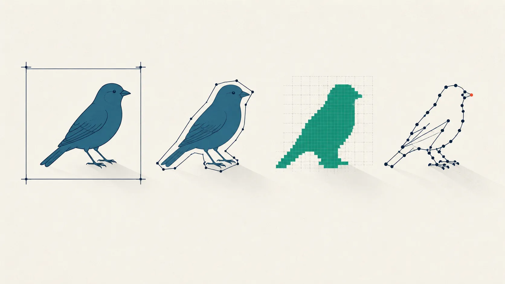 Image & Multimodal Annotation
Image Annotation Types: Cost vs Precision, Explained
Bounding box, polygon, semantic vs instance vs panoptic masks, or keypoints? Compare image annotation types by cost, precision, and downstream task.
 Image & Multimodal Annotation
Dice vs IoU vs Hausdorff: Segmentation Metrics Explained
Dice vs IoU, the Jaccard index, and Hausdorff distance compared: formulas, the Dice-IoU identity, and when overlap metrics mislead. See which to report.
Put this into practice
Tagaroo turns any rating scale or coding scheme into a guided annotation workflow—with inter-rater reliability computed as you go.